Construction of Optimization Problems¶

This package targets an important family of problems in machine learning and data analytics, namely, (regularized) empirical risk minimization. Such problems can generally be expressed as:

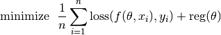
$\text{minimize } \ \frac{1}{n} \sum_{i=1}^n \mathrm{loss}(f(\theta, x_i), y_i) + \mathrm{reg}(\theta)$

This objective is comprised of two parts: the data terms, which is the average loss evaluated at all samples, and a regularization term that encourages lower model complexity. In particular, each loss term compares the output of the predictor f and a desired output. To sum up, three components are involved: predictor, loss function, and regularizer.

This package provides facilities to construct these components respectively, and the SGD solver will take these components as inputs.

Predictors¶

All predictors in this package are organized with the following type hierarchy:

abstract Predictor

abstract UnivariatePredictor <: Predictor      # produces scalar output
abstract MultivariatePredictor <: Predictor    # produces vector output

Methods¶

The following methods are provided for each predictor type. Let pred be a predictor.

predict(pred, theta, x)¶

Evaluate and return the predicted output, given the parameter theta and the input x.

The form of the output depends on both the predictor type and the input.

predictor type	input `x`	output
`UnivariatePredictor`	a vector of length `d`	a scalar
`UnivariatePredictor`	a matrix of size `(d, n)`	a vector of length `n`
`MultivariatePredictor`	a vector of length `d`	a vector of length `q`
`MultivariatePredictor`	a matrix of size `(d, n)`	a matrix of size `(q, n)`

Note: for multivariate predictors, the output dimension q need not be equal to the input dimension d.

scaled_grad!(pred, g, c, theta, x)

Evaluate scaled gradient(s) at given sample(s), writing the resultant gradient(s) to g.

When x is a vector that represents a single sample, it computes c times the gradient and writes the resultant gradient to a pre-allocated vector g.

When x is a matrix that comprises n samples (each being a column), then c must be a vector of length n, it computes the linear combination of the gradients evaluated at the given samples, using the values in c as coefficients. Likewise, the resultant accumulated gradient is written to g.

g should be of the same size as theta.

Note: this function is mainly used by the internal of the optimization algorithms.

The package already provides several commonly used predictors as follows. Users can also implement customized predictors by creating subtypes of Predictor and implementing the methods above.

Linear predictor¶

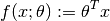
A linear predictor is a real-valued linear functional $f: \mathbb{R}^d \rightarrow \mathbb{R}$ , given by

$f(x; \theta) := \theta^T x$

In the package, a linear predictor is represented by the type LinearPredictor:

type LinearPredictor <: UnivariatePredictor
end

Affine predictor¶

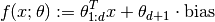
An affine predictor is a real-valued linear functional $f: \mathbb{R}^d \rightarrow \mathbb{R}$ , given by

$f(x; \theta) := \theta_{1:d}^T x + \theta_{d+1} \cdot \mathrm{bias}$

Note that the parameter $\theta$ is an d+1-dimensional vector, which stacks the coefficients for features and a coefficient for the bias.

In the package, an affine predictor is represented by the type AffinePredictor:

type AffinePredictor{T<:FloatingPoint} <: UnivariatePredictor
    bias::T
end

AffinePredictor{T<:FloatingPoint}(bias::T) = AffinePredictor{T}(bias)
AffinePredictor() = AffinePredictor(1.0)

Multivariate linear predictor¶

A multivariate linear predictor is a vector-valued linear functional $f: \mathbb{R}^d \rightarrow \mathbb{R}^q$ , given by

$f(x; \theta) := \theta^T x$

The parameter $\theta$ is a matrix of size (d, q).

In the package, a multivariate linear predictor is represented by the type MvLinearPredictor:

type MvLinearPredictor <: MultivariatePredictor
end

Multivariate affine predictor¶

A multivariate affine predictor is a vector-valued linear functional $f: \mathbb{R}^d \rightarrow \mathbb{R}^q$ , given by

$f_i(x; \theta) := \theta_{1:d, i}^T x + \theta_{d+1, i} \cdot \mathrm{bias}, \ \forall i = 1, \ldots, q$

The parameter $theta$ is a matrix of size (d+1, q).

In the package, a multivariate affine predictor is represented by the type MvAffinePredictor:

type MvAffinePredictor{T<:FloatingPoint} <: MultivariatePredictor
    bias::T
end

MvAffinePredictor{T<:FloatingPoint}(bias::T) = MvAffinePredictor{T}(bias)
MvAffinePredictor() = MvAffinePredictor(1.0)

Note: In the context of classification, one should directly use the value(s) yielded by the linear or affine predictors as arguments to the loss function (e.g. logistic loss or multinomial logistic loss), without converting them into class labels.

Loss Functions¶

All loss functions in the package are organized with the following type hierarchy:

abstract Loss

abstract UnivariateLoss <: Loss       # for univariate predictions
abstract MultivariateLoss <: Loss     # for multivariate predictions

Methods¶

All univariate loss functions should implement the following methods:

value_and_deriv(loss, u, y)¶: Compute both the loss value and the derivative w.r.t. the prediction and return them as a pair, given both the prediction u and expected output y.

All multivariate loss functions should implement the following methods:

value_and_deriv!(loss, u, y): Compute both the loss value and the derivatives w.r.t. the vector-valued predictions, given both the predicted vector u and the expected output y. It returns the loss value, and overrides u with the partial derivatives.

This package already provides a few commonly used loss functions. One can implement customized loss functions by creating subtypes of Loss and providing the required methods as above.

Squared loss¶

The squared loss, as defined below, is usually used in linear regression or curve fitting problems:

$loss(u, y) = \frac{1}{2} (u - y)^2$

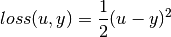
It is represented by the type SqrLoss, as:

type SqrLoss <: UnivariateLoss
end

Hinge loss¶

The hinge loss, as defined below, is usually used for large-margin classification, e.g. SVM:

$loss(u, y) = \max(1 - y \cdot u, 0)$

It is represented by the type HingeLoss, as:

type HingeLoss <: UnivariateLoss
end

Logisitc loss¶

The logistic loss, as defined below, is usually used for logistic regression:

$loss(u, y) = \log(1 + \exp(-y \cdot u))$

It is represented by the type LogisticLoss, as:

type LogisticLoss <: UnivariateLoss
end

Multinomial Logistic loss¶

The multinomial logistic loss, as defined below, is usually used for multinomial logistic regression (this is often used in the context of multi-way classification):

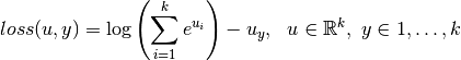
$loss(u, y) = \log\left(\sum_{i=1}^k e^{u_i} \right) - u_y, \ \ u \in \mathbb{R}^k, \ y \in {1, \ldots, k}$

Here, k is the number of classes. This loss function should be used with a k-dimensional multivariate predictor.

It is represented by the type MultiLogisticLoss, as:

type MultiLogisticLoss <: MultivariateLoss
end

Regularizers¶

Regularization is important. Using regularization can ensures numerical stability and often improves the generalization performance of a model. In this package, regularization is done through regularizers, which can be understood as functionals that yield a cost value given a parameter.

Methods¶

All regularizers are subtypes of an abstract type Regularizer, and should implement the following methods:

value_and_addgrad!(reg, g, theta)

Compute the regularization value and the gradient at the parameter theta. It returns the regularization value and writes the gradient to a pre-allocated array g.

The size of g should be equal to that of theta.

The package provides some commonly used regularizers.

No regularization¶

In certain cases, e.g. with a large sample set, people may choose to not use regularization. We provide a type NoReg, defined below, to indicate no regularization.

type NoReg <: Regularizer end

In SGD algorithms, if no regularizer is explicitly specified, NoReg() will be used by default.

Squared L2 norm¶

The squared L2 norm regularizer is defined as

$r(\theta) = \frac{c}{2} \|\theta\|_2^2$

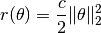
It is represented by the type SqrL2Reg, as:

type SqrL2Reg <: Regularizer
    coef::Float64
end

L1 norm¶

The L1 norm regularizer is defined as

$r(\theta) = c |\theta|_1$

It is represented by the type L1Reg, as:

type L1Reg <: Regularizer
    coef::Float64
end

This regularizer is often used for sparse learning, e.g. LASSO.

Elastic regularizer¶

The elastic regularizer is defined as a combination of L1 norm and squared L2 norm, as:

$r(\theta) = c_1 \|\theta_1\|_1 + c_2 \|\theta_2\|_2^2$

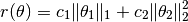
It is represented by the type ElasticReg, as:

type ElasticReg <: Regularizer
    coef1::Float64
    coef2::Float64
end

This is the regularizer used in the well-known algorithm Elastic Net.